The Modern Taylor Method Solver of ODEs:
The Taylor Center
Keywords: ODE Solver, Taylor Solver, Taylor Method, Taylor Series, Power Series Method, Clean Numerical Simulation, Adjoint equations, Numeric Integration, High Accuracy, Ultimate Accuracy, Finite Step, Dynamic Graphics, 3D Stereo, 3D Cursor, Trajectories, Interactive environment, Windows, Linux.
The Modern Taylor Method is a descender of its classical counterpart. It is an efficient method for numerical integration of the Initial Value Problems (IVPs) for holomorphic Ordinary Differential Equations (ODEs) whose Right Hand Sides are general elementary functions.
The Taylor Center (Tcenter) is a 32-bit application for PCs, capable of addressing up to 4GB of memory on all 32-bit versions of Windows from NT and XP (1996) to the current Windows 11 (2026), and hopefully further on.
What distinguishes it from all other numerical methods for ODEs is that …
· The Taylor method computes the increments of the solution with principally unlimited order of approximation so that the integration step must not approach zero whichever high accuracy is specified. That is possible because the method performs the automatic differentiation – exact computing of the derivatives up to any desired order n, allowing to obtain the Taylor series of any length for the solution components.
· The Taylor method does not use any finite difference formulas such as f'(t) ≈ ( f(t+h) – f(t) ) / h prone to (catastrophic) subtraction error with float point numbers of fixed length.
· The Taylor Center utilizes the 80-bit float point type extended with 63-bit mantissa generic for the processor X87 FPU – while other numeric programs (such as Mathematica®, Maple®, Matlab®, Simulink® with MathWorks®) use the 64-bit float type double with 52-bit mantissa for their generic float point computation. (The emulated unlimited precision in those systems is several orders of magnitude slower than the generic float point processing).
According to the concept of Clean Numerical Simulation of integration, such a method must …
· Implement the Taylor method integration,
· Employ the maximum available floating-point representation,
· Check the accuracy of integration.
According to these criteria, the Taylor Solver introduced here is a Clean Numerical Simulation Method.
|
To install this program for Windows called TCenter, click here, then download the file: Save, rather than Open it in your browser. Unzip it entirely (right click choosing Extract all) and keep it in an empty folder, TCenter.exe being the only executable to run. (This application does not modify Windows registry, nor does it need an installer or uninstaller). Preserve these files and sub-folder structure (in order that the program work properly). See a short guide navigating you through the DEMO. You can also download the full User Manual (in MS Word doc format), or the articles (in pdf) published in the Proceedings CSC 2005 , DMS 2007 , and in CODEE Journal, September 2012. For pedagogical use and courseware see the Exploratorium. |
From the algorithmic point of view, this software parses the right-hand sides of the ODEs and auxiliary equations, and compiles them into a sequence of pseudo instructions of Automatic Differentiation. Then the programmatic emulator of those instructions runs them evaluating the derivatives and integrating the Initial Value Problem.
To make inquiries, please contact Alexander Gofen at alex@taylorcenter.org .
With the current version of the product, you can:
- Specify and study the Initial Value Problems for virtually any system of holomorphic ODEs in the standard format (whose Right-Hand Sides are general elementary functions), meaning a system of explicit first order ODEs, derivatives in the left-hand sides and arithmetic expressions in the right hand. The standard elementary functions, numeric and symbolic constants and parameters may be used;
- Enter arithmetic expression in the standard Pascal syntax either through the editor windows, or via the Polynomial Designer for cumbersome 2nd degree multivariate polynomials;
- Perform numerical integration of Initial Value Problems with an arbitrary high accuracy for the standard 64 bit mantissa in PCs, along a path without singularities, while the step of integration remains finite and does not approach zero (presuming the order of approximation or the number of terms could increase to infinity with the length of mantissa unlimited);
- Apply an arbitrary high order of approximation (by default 30), and get the solution in the form of the set of analytical elements – Taylor expansions covering the required domain;
- Study Taylor expansions and the radius of convergence for the solution at all points of interest up to any high order. An upper limit for the terms in the series is as high as 104932 implied by the Intel generic 10 byte float point type extended with 64-bit mantissa (contrary to the reduced 8 byte type double with 52 bit mantissa in Microsoft C++ as the highest precision);
- Perform integration either "blindly" (observing only the numerical changes), or graphically visualized.
- Graph color curves (trajectories) for any pair of variables of the solution – up to 200 on one screen – either as plane projections, or as 3D stereo images (for triplets of variables) to view through anaglyphic (red/blue) glasses. The 3D cursor with audio feedback enables "tactile" exploration of the curves literally hanging in "thin air";
- Graph non-planar curves as though tubes of a required thickness implementing the proper skew resolution at points of illusory intersections;
- "Play" dynamically the near-real time motion along the computed trajectories either as 2D or 3D stereo animation;
- Graph the enhanced field of directions (a Phase portrait), actually the field of curvy segments, whose length is proportional to the radius of convergence.
- Dynamically plot a triangle based on the 3 bullets of the first 3 trajectories visualizing the moments of syzygy (i.e. when the bodies in the 3-body problem are collinear);
- Dynamically plot the 3 moving axes of coordinates fixed within a moving solid body (or the respective tetrahedron) based on the 4 bullets in order to visualize the motion of a solid body in 3D;
- Graph monomials of Taylor expansions as bar diagrams and vary the step h observing its effect on the bell shape bulge;
- Terminate the integration either after a given number of steps, or until an independent variable reaches a given terminal value exactly, or until the control function reaches a given terminal value approximately, or when a dependent variable reaches a given terminal value exactly in ODEs in a different state (as explained in the next item);
- Automatically generate the ODEs and switch integration between several states of ODEs (adjoint equations) defining the same trajectory, but with respect to different independent variables. For example, it is possible to switch the integration in respect to t to that by x, or by y in order to reach the terminal value (or zeros) of a former dependent variable (x, or y). In particular, if the initial (guess) value is a nonzero and the terminal value is set to zero, the root (the zero) of the solution may be obtained directly without iterations;
- Automatically generate and simultaneously integrate an array of Initial Value Problems for an array of initial vectors. The solutions of these IVPs are displayed in one plot resembling a phase portrait. An array of IVPs considered as an IVP with an indefinite parameter helps to estimate the solution of certain boundary value problems;
- Automatically perform massive sequential integration of an array
of Initial Value Problems for an
array of initial vectors prepared in advance. The results of the massive
computation are saved into a file.
- Integrate piecewise-analytical ODEs;
- Specify different methods to control the accuracy and the step size;
- Specify accuracy for individual components either as an absolute or relative error tolerance, or both;
- Explore a collection of meaningful examples supplied with the package such as the problem of Three and Four Bodies. Symbolic constants and expressions allow parameterization of the equations and initial values, along with trying different initial configurations of special interest.
- Automatically generate ODEs for the classical Newtonian n-body problem for n up to 99, and then integrate and explore the motion. In the case of n=99 there are 595 ODEs, 19404 auxiliary equations, compiled into over 132000 variables and over 130000 AD processor's instructions: a "heavy duty" integration!
- Use a DLL (for any programming languages under Windows accepting the real 80 byte type extended). This DLL (without using the Taylor Center) provides functions for computing the vector-function of a solution of ODEs earlier obtained with the Taylor Center. The DLL implements the optimized (Horner algorithm) for computation of the desired vector function using the polynomial expansions obtained from the Taylor integration and saved as a binary file (to re-use the integration results obtained in the Taylor Center in other user applications);
- Integrate a few special instances of singular ODEs having regular solutions at the points of the so called "regular singularities".
In particular, the Demo includes fascinating examples of the so called choreography for the 3 body problem: 345 of them (courtesy of Dr. Carles Simò), plus 204 cases of periodic orbits of unusual shapes (courtesy of Ana Hudomal). Click here to learn more about the Choreographies of N-body problem and how to "feed" their ODEs and initial values into the Taylor Center, plot the curves and play the motion in the real-time mode: all in the same place. Similarly, click here for playing with the periodic orbits for the 3 body problem from the list of Ana Hudomal. These orbits are closed curves (as intuitively expected from periodic orbits). Here however you may see the newly discovered periodic orbits which are finite curved segments, whose extremes are resting points in the 3-body problem, so that the bodies periodically fulfill a free fall along these segmented orbits (the data was kindly provided by Xiaoming LI and Shijun LIAO). Another recent fascinating example of the four body non-planar trajectories inscribed in a cube discovered by Cris Moore & Michael Nauenberg is incorporated too. Here is the list of brief explanations for all several hundreds samples pre-loaded with the program.
As of now (and in foreseeable future), the Taylor Center will remain a 32-bit application
run on the x87 FPU. This processor was designed to address only 32 bit
address space, i.e. no more than 4 Gb memory, or 400 millions of variables and
their expansions (as 10 byte float point numbers).
In order to randomly address a memory space larger than 4 Gb, Intel (and other companies) enhanced the x87 FPU processor by adding a set of instruction SSE capable to randomly access a 64 bit address space. However in doing so, Intel designed the SSE instructions to operate only on the 8 byte data types abandoning the 10 byte type extended. Though it is logically possible to expand the addressing ability of the x87 FPU by combining its 32-bit instructions with the SSE instructions to randomly address the 64 bit memory space, such a trick prohibitively slows the overall operation speed of x87 FPU on the 10 byte type.
For the program like the Taylor Center it's crucial to operated with the highest precision available in a processor. Therefore, with such a design blunder by Intel, it makes sense to maintain the Taylor Center only as a 32 bit application operating at the x87 FPU with the 10 byte type at the highest speed.
The memory consumption
depends on the number of variables VarNum (a function of the number of
ODEs and their complexity) and on the specified Order of approximation.
If the expansions are not stored, the program takes 2*VarNum*Order*10
bytes of memory. If the expansions in P points are stored, it additionally
requires P*VarNum*Order*10 bytes.
A benchmark for the 10 body planar problem comprised of 2*(10+10)+1=41
ODEs and 10*9/2*(2+1)=135 auxiliary equations, which are parsed into 811 AD
instructions. For this problem 10000 steps of integration took 32 s (or 3.2 ms
per step) on 2.4 GHz Pentium with polynomial expressions spelled out, and it
took 29 s (or 2.9 ms per step) with polynomial expressions encoded.
A benchmark for the 99 body spatial problem comprised of 3*(99+99)+1=595
ODEs and 99*98/2*(3+1)=19404 auxiliary equations, 100 steps took 65 s with
polynomial expressions spelled out, and took 42.5 s with polynomial expressions
encoded.
An accuracy benchmark for the so-called Pythagorean triangle 3-body
problem (Pythagor.scr) demonstrates how successfully this software overcomes
near catastrophic cancellation errors emerging during close approach of the
bodies in this particular problem. While fixed order methods required the Levi-Civita's
regularization of binary collisions in order to complete the integration, this
software successfully integrated this problem without regularization as a
general Newtonian 3-body problem.
Generally for each system of ODEs there exists such a small value of the
accuracy requirement, that at this high accuracy the Taylor methods beats any
fixed order method due to the unlimited order of approximation in the Taylor
method.
The future version will include the following:
- It will be supplied not only as the Taylor Center GUI executable, but also as the separate Delphi component (to include them directly in Delphi projects);
- To integrate IVPs in complex variables along an arbitrary path in a complex plane.
- The set of the internal differentiation instructions will be translated into the machine code – to reach the highest possible speed for massive computations. (Meanwhile it is an emulator written in Delphi which runs these instructions). Also, the set of the internal AD instructions may be translated into instructions in Pascal, C or Fortran to be further compiled and linked with other applications;
Here is how the front panel of the Taylor Center looks like:
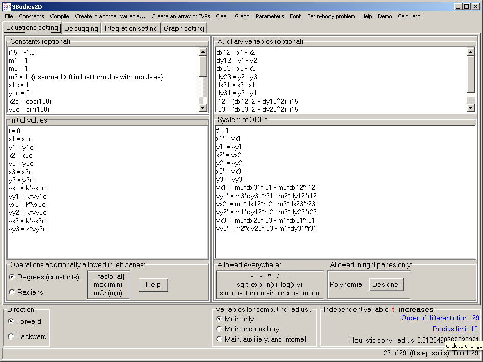
for the Lagrange case of the 3-body problem:
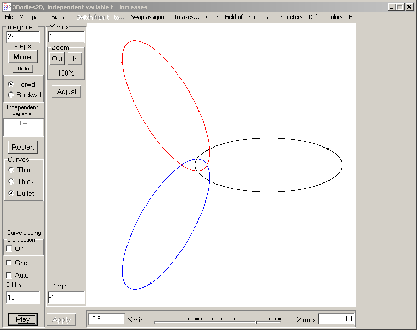
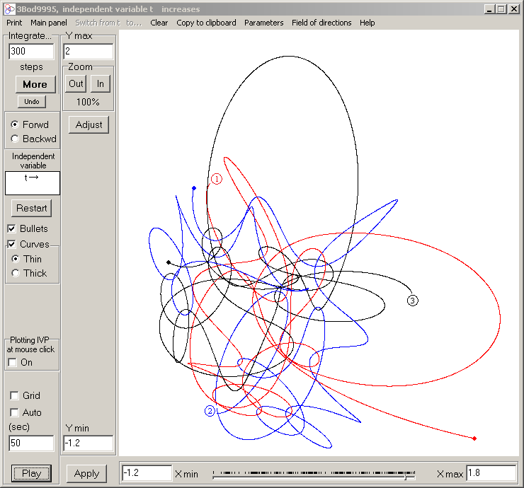
And here are the trajectories of a slightly disturbed Lagrange case of the 3-body problem (Demo/Three bodies/Disturbed/2D). However, there is a dramatic difference between viewing a still image like this vs. dynamically evolving real time motion displayed in the running Taylor Center. In the Demo you will be fascinated to watch all possible pairs of the three bodies coupling randomly in turn with acceleration or deceleration.
This software was used for studying several challenging cases in the n-body problem listed in the Exploratorium. For example, here is a beautiful picture of the special case of the 3-body problem known as the spatial Sitnikov case
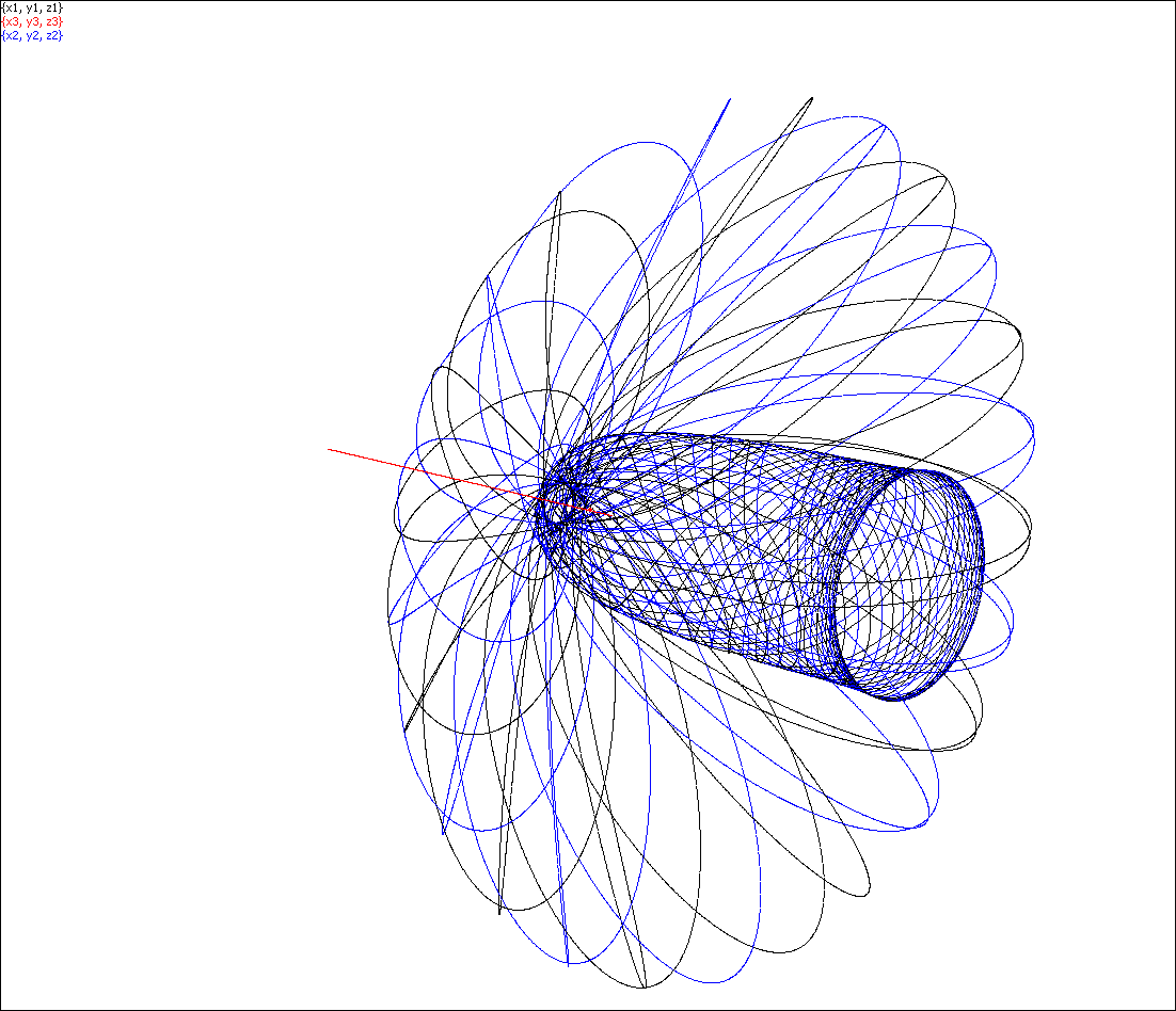
and other pictures of the Sitnikov case may be seen here.
Generally, in this software, the visualization is encoded in short script files: scalable for any resolution, duration, and the highest refresh rate. Yet the software can also save frames ready for the movie format. The movies (though not so robust) are platform-independent and may run without installation of this software. For example, here are such movies for the above-mentioned Sitnikov case, or for the new study of the Double pendulum. In the problem of a rolling disk, the disk is outlined with 10 points and a trajectory of the point of touch, as showed in these two movies: the 8-shape and 4 petals (credit to D. Garanin).
Here is a Double spiral (Demo/Spirals/Double spiral) – a solution of the system
x' = x²
- y²+ 2xy - x -3.5y + 1,
x(0)=0.1
y' = -x² + y² + 2xy - y +3.5x - 1,
y(0)=0
corresponding to one complex ODE z' = (1 - i)z² + (-1
+ 3.5i)z + 1 - i, z = x + iy. Similarly to the previous
example, it is one thing to see this Double Spiral as a static
image
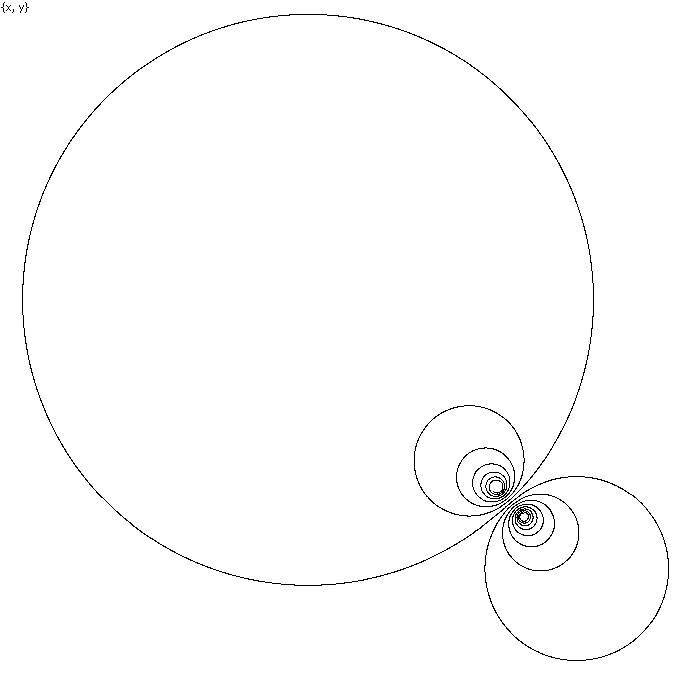
It is quite different thing to watch the real-time motion along this
spiral observing that every lap of the spiral takes exactly the same time to
run (with a huge acceleration in big laps), as it follows from the complex analysis. Beside running the
program (Demo/Spirals/ Double spiral), this particular example is also
recorded as a movie runnable at any platform
without installing the program.
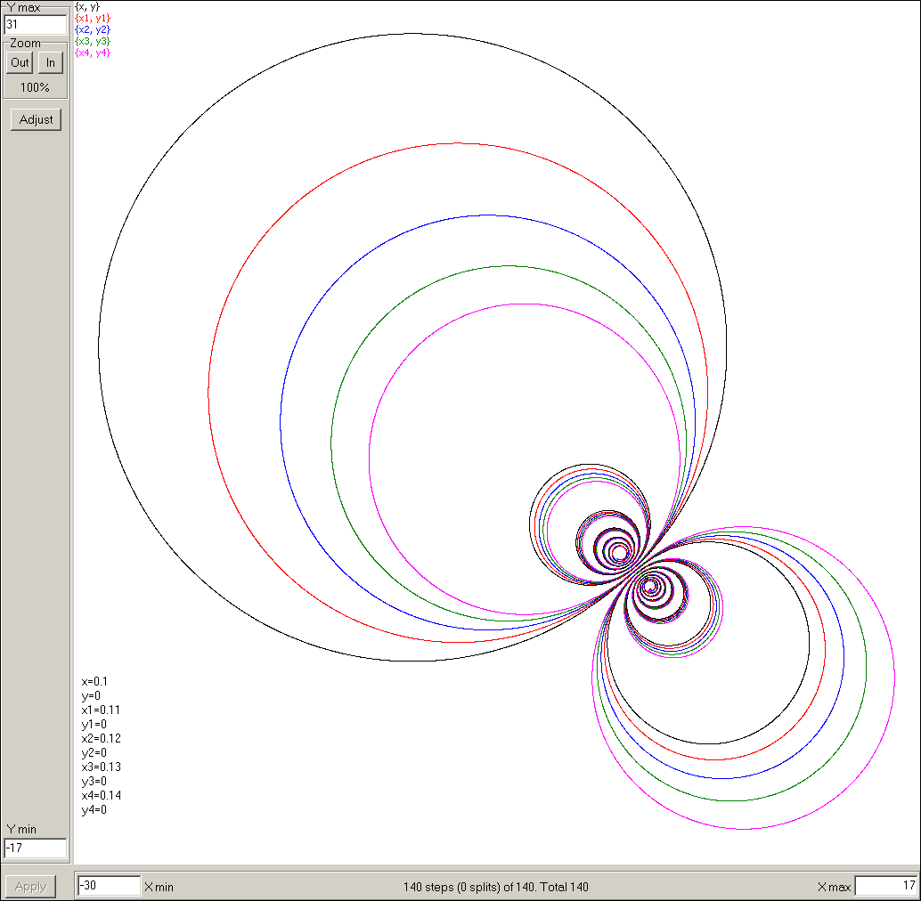
And here is an array of 5 Initial Value Problems integrated simultaneously for
the same system of ODEs with various initial values:
In cases when the goal is to study and visualize properties of a particular Taylor expansion for one of the variables, this software provides the Taylor profile window
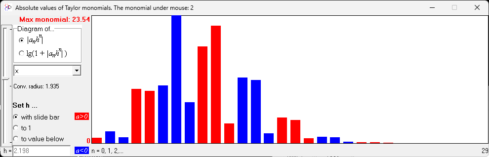
which graphs a diagram of the values of the Taylor monomials |anhn| allowing to observe the change of the profile for various h controlled by the slide bar at the left.
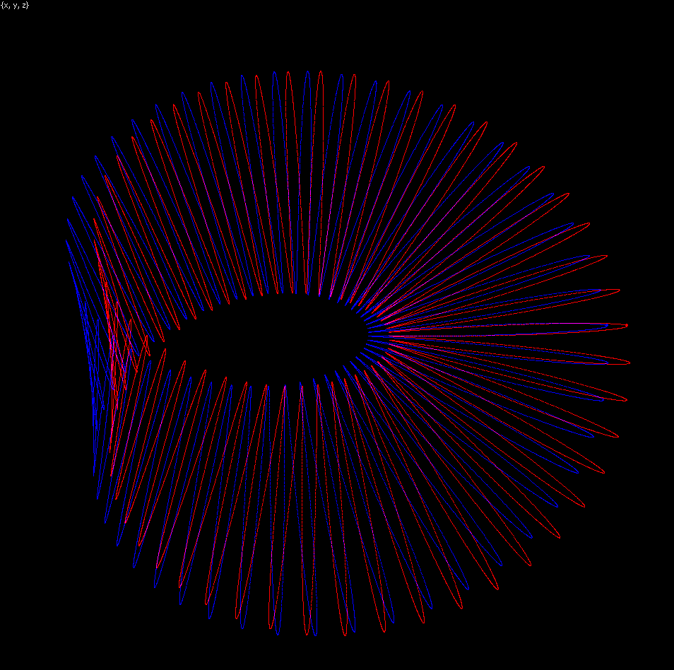
The unique feature of this software is that 3D viewing and real time animation is implemented also in stereo mode. To view stereo images, you need anaglyphic Red/Blue glasses (Left - Red, Right - Blue). Such glasses may be ordered here: look for a Red/Blue type (not Red/Cyan).
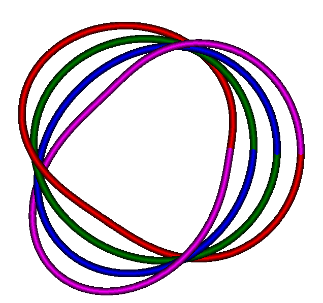
If you have the anaglyphic glasses, click to view 3D stereo images (and explanation of the optimal viewing conditions). You may view non-planar curves also in conventional axonometry projection (where their spatial properties are lost). However, in order to improve axonometric view of such curves, this software can draw them as though tubes of a required thickness implementing the proper skew resolution at points of illusory intersections like in this family of curves representing the double Möbius surface outline:
This software offers several tricks for outlining 3D surfaces. The image above is based on visualizing one of two families of the internal coordinate lines of the Möbius surface. Another way of visualizing single Möbius surface is based on the sine wave with a short wavelength: here in 3D stereo or in tubular graphic below
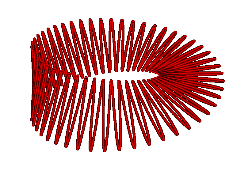
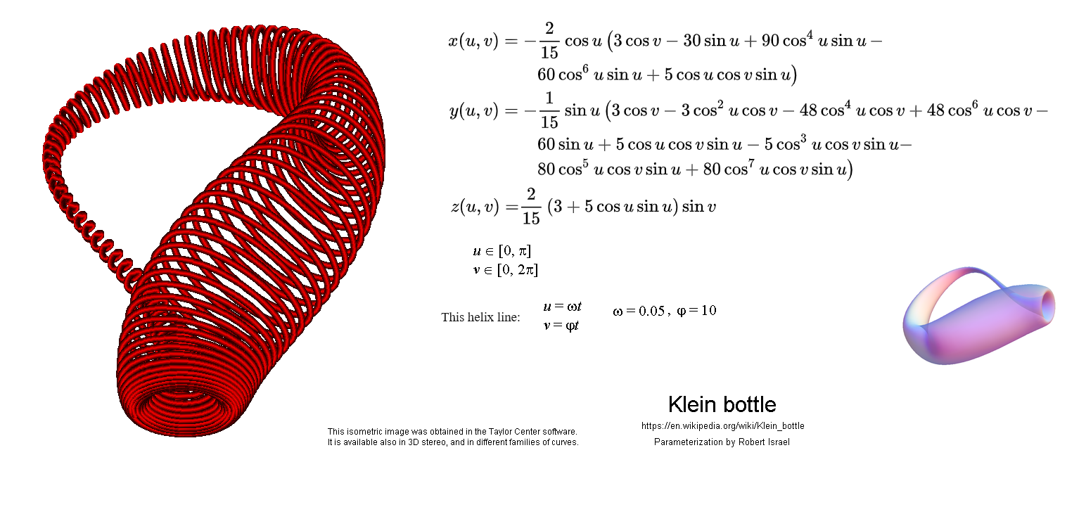
One more approach of outlining is based on helix, say for outlining tori, or the Klein bottle below
You may also construct and display an enhanced field of directions or a phase portrait for selected pairs of variables built not with small vectors, but rather with analytic elements i.e. curvy strokes representing finite pieces of trajectories obtained in multi-step integration at points of a grid or at arbitrary points of your choice. Due to the high order of the Taylor method, these strokes are typically long enough to represent the near continuous family of the solutions or the phase portrait like that below for the system:
x' = -y + 2x2 +
xy - y2
y' = x + x2 - 3xy
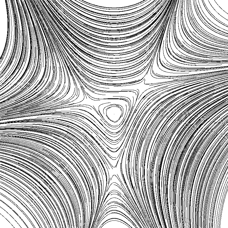
This is a phase portrait explaining the behavior of a spinning wingnut in weightlessness – the so called Dzanibekov effect, covered in the extensive article on the Rigid body motion here:
PhasePort.png)
And here is another beautiful phase portrait made by this software for a system (credit to John H. Hubbard and Beverly H. West)
x'
= 1
y' = y2 - x
The image below depicts the two curves of this phase
portrait near the separatrix. The initial values of these curves differ only in
the last binary digit of their 64 bit mantissa:
x%5e2-t.png)
Normally, in order to populate and reach the
maximal accuracy in 64 bit mantissa, 19 or 20 significant decimal digits
suffice. The routine converting real decimal numbers into this float binary format
may take also extra decimal digits, yet the binary result will be rounded to 64
significant binary digits anyway. In this example the two decimal numbers are
represented with 22 decimal digits, however the difference between their binary
form is exactly one last bit of the mantissa (the goal set in this experiment).
This smallest difference in the initial values however was enough to finally
direct the black curve upward yet the red curve downward, demonstrating the ultimate
accuracy of integration for this 64-bit mantissa real type. The relative error
tolerance in this case was set to 10-25 < 10-19 meaning that at every of 80 finite steps, all 64 binary digits of the
result were true, so that the highest accuracy at every step (in a format with
64 bit mantissa) was achieved.