Three body free fall periodic orbits:
new remarkable features
This text with more detales in pdf
The related gallery of orbits
By Alexander Gofen
December, 2021
The three body motion under the Newtonian gravitation has been intensively
studied since Isaac Newton over 300 years, still presenting a challenge.
Besides the special cases of elliptic (and other conics) by Euler and Lagrange,
no other versions of regular motion of three bodies were known for a long time.
Since emergence of computers, also numeric simulations were used to explore the
orbits for various initial settings, most of which generated a chaotic motion.
So more surprising were discoveries of remarkable types of
plane periodic motion of three bodies obtained in computer assisted researches.
Such were the discovery of ...
- Choreography, when three bodies move along the same periodic curve one after the other;
- Periodic and relatively periodic orbits;
- Free fall periodic orbits meaning that three bodies have zero velocity at the initial moment: the topic of this workshop.
In 2018
Xiaoming Li and Shijun Liao [1-3] discovered hundreds of settings for initially
resting three bodies making periodic motion: i.e. the bodies started at the
given rest points, and returned back to their initial rest points after motion
along sophisticated orbits during a period T.
We call the moments of time when all three bodies rest the
break points paying attention to the triangular formation at the moments of
rest.
It's worth particular mentioning that Xiaoming Li and Shijun
Liao [2, 3] developed and ran their search of various initial settings of the
rest points with the only goal to figure out solutions having periods. They did
it by watching for the values of the target function whether its values are
close to zero (with the given threshold).
However, despite setting the goal of obtaining merely periodic solutions ending
in the same initial points, all their 30 solutions for equal masses
demonstrated some additional properties not specified in the search criterion:
1. As pointed out by the authors [3], in all those discovered periodic trajectories, the initial rest formations at the moments kT (k=0, 1, ...) happened to be not the only one. In every periodic lap of the trajectory the number of break points was exactly 2: namely the initial moment and the moment T/2 where all three bodies come to rest, but at a formation differing from the initial one. That meant that ...
2. The three bodies oscillated between two formations: the initial and second set of the rest points (specific for each simulation).
Though the authors did mention it [3], they did not provide any explanation for
this unexpected "side effect" taking place in all 30 cases.
We discovered other even more remarkable "side effects"
not specified as a search criterion too. They appear as certain exact
relations, though not in all, but only in a few of the 30 simulations.
Emergence of such uninvited properties in a massive search is puzzling. These
properties are reported in the section "Newly discovered properties".
The fact that the properties 1, 2 took place even though
never specified as a search criterion has an explanation, which follows from
the next Theorem (by Richard Montgomery).
Theorem: Free fall periodic orbits have exactly two sets (two
formations) of rest points so that the bodies oscillate between them.
This Theorem explains why the search process of periodic
orbits starting with a break point delivered the orbits all having the second
break points.
All such orbits are cataloged and displayed as movies at the
authors' site [1]. The first 30 simulations in the table present the cases of
all three masses equal 1. These simulations also come with the free installation
of the software Taylor Center (where you can watch them in real time with the
resolution much higher than in the movies [1]).
In the next section we report more new properties, taking
place, however, not in all 30 of the above-mentioned orbits. Those properties
were discovered by chance in numeric experiments with the 30 simulations
performed and verified with the Taylor Center software.
The new properties.
Here we summarize the newly discovered properties taking
place in 12 of the 30 orbits.
The Table 1 below shows in which of the 30 simulations [1]
these earlier unknown properties take place.
We consider two triangular formations of the 3 bodies: the
initial △ABC at the moment t=0 and the second △A′B′C′ at the moment t=T/2, where △ABC and △A′B′C′
are congruent with or without reflection. This means the equality of the
corresponding angles ∠A=∠A′,
∠B=∠B′,
∠C=∠C′.
Let the bodies #1, #2, #3 at the initial moment reside
correspondingly at the vertices A, B, C of the △ABC. Their trajectories, however, may not necessarily lead to the
corresponding vertices A′, B′, C′ of the △A′B′C′, as some simulations below
demonstrate. Among the data collected by the research program, there are the
permutations (αβγ), where the identity permutation is denoted
Id=(123). If the trajectories of the bodies #1, #2, #3 (black, red, and blue)
lead from the vertices A, B, C to the corresponding vertices A′, B′,
C′ (no matter whether △A′B′C′
is a reflection of △ABC), the corresponding permutation is Id;
otherwise the permutation differs from Id.
These newly discovered properties in 12 of the 30 orbits are
the following:
3. In the moments (1/4)T and (3/4)T the bodies are either
in syzygy (item 5), or they form an isosceles triangle (item 6).
4. The triangle formation at the second break point (1/2)T is
congruent to the initial triangle.
5. In 3 of the 12 orbits in the moments (1/4)T and (3/4)T
the second triangle is a result of 180° rotation of the initial triangle so
that both triangles and respective parts of orbits are symmetric over the
central point lying on the syzygy, one of the bodies being in the middle. At
that, the three vectors of the velocities in the moments (1/4)T and
(3/4)T are reciprocally parallel. However...
6. In the remaining 9 orbits the edges are not parallel, and both
triangles are in the relation of reflection, i.e. the two respective parts of
orbits are symmetric over some line of symmetry, which, however, is not
necessarily the line of syzygy. Specifically...
7. If there is no permutation (i.e. Id takes place), then in the
moments (1/4)T and (3/4)T the 3 bodies are in syzygy on the line
of symmetry, otherwise in the moments (1/4)T and (3/4)T the
bodies are not in syzygy, forming an isosceles triangle.
The properties (3-7) are not mentioned in the original
sources [1-3], and therefore they are new. Unlike the properties (1-2) proven
to take place in any free fall periodic orbit, at the moment it's not known the
conditions leading to the 12 cases of congruency discussed here.
|
At T/2 |
At T/4 |
|||||
|
# |
Congruency |
Parallel edges |
Symmetry |
Permutation |
Isosceles |
Syzygy |
|
1 |
||||||
|
2 |
||||||
|
3 |
||||||
|
4 |
Yes |
Reflection |
(321) |
Yes |
||
|
5 |
||||||
|
6 |
Yes |
Reflection |
(321) |
Yes |
||
|
7 |
||||||
|
8 |
Yes |
Reflection |
(123) |
Yes |
||
|
9 |
||||||
|
10 |
Yes |
Reflection |
(123) |
Yes |
||
|
11 |
||||||
|
12 |
||||||
|
13 |
||||||
|
14 |
Yes |
Yes |
Central |
(213) |
Yes |
Yes |
|
15 |
Yes |
Yes |
Central |
(213) |
Yes |
Yes |
|
16 |
||||||
|
17 |
||||||
|
18 |
Yes |
Reflection |
(123) |
Yes |
||
|
19 |
Yes |
Reflection |
(132) |
Yes |
||
|
20 |
||||||
|
21 |
||||||
|
22 |
Yes |
Reflection |
(123) |
Yes |
||
|
23 |
||||||
|
24 |
||||||
|
25 |
Yes |
Reflection |
(123) |
Yes |
||
|
26 |
||||||
|
27 |
Yes |
Yes |
Central |
(132) |
Yes |
Yes |
|
28 |
||||||
|
29 |
Yes |
Reflection |
(123) |
Yes |
||
|
30 |
||||||
How the triplets of initial points were obtained
As explained in [1-3], the
authors fixed the points q1 = (-0.5, 0), q2 = (0.5,
0), while the goal of the search algorithm was to obtain points q3 such
that the target function be near zero with the specified accuracy. Below is a
scattered graph for the 30 points q3 obtained in the search process [1-3]:
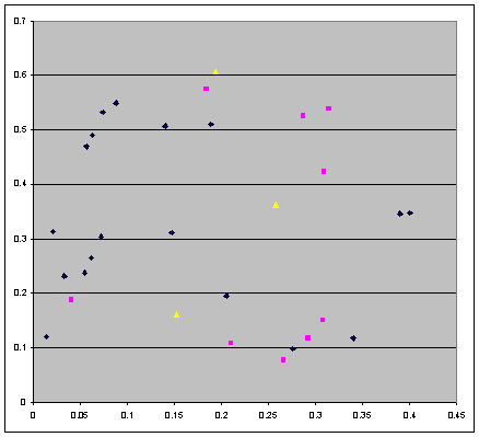
Figure 1. The 30 values for the third initial point q3 obtained in a search algorithm
The three yellow points correspond to the cases of the central symmetry, the 9
magenta points correspond to the cases of reflection, and the remaining blue
points correspond to the orbits with no special properties. This graph does not
reveal any remarkable pattern. There is no mentioning in [1-3] whether the
search algorithm delivered all existing points q3 in the
given bounded area of search, and whether the number of points q3 is
finite or infinite.
Some illustrations
Here are several illustrations of the
characteristic cases mentioned above presented in high resolution of the Taylor
Center software. All the 30 simulations may be viewed also in real time
animation within this software as explained here or as still images here.
In the pictures below the trajectories are color coded as A→A', B→B', C→C'
where primed point is the second point of rest for the respective initial
point. However the edges and angles of the triangle ∆ABC at the initial
moment may not necessarily match the edges and angles of the second triangle
even when both triangles are congruent: they can flip in various manner as the
consequence of the motion.
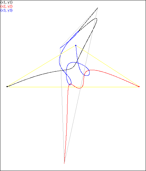
Simulation #1: the second triangle and the first are dissimilar.
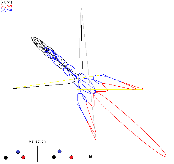
Simulation #18: the second triangle and the first are congruent.
AB = 1,
AC = 0.718590490501491,
BC
= 0.309097112311281
A'B' = 1.00000000170251,
A'C' =
0.718590493477556, B'C' = 0.309097111598536
A'B'/AB =
1.00000000170251, A'C'/AC =
1.00000000414153 , B'C'/BC=
0.999999997694106
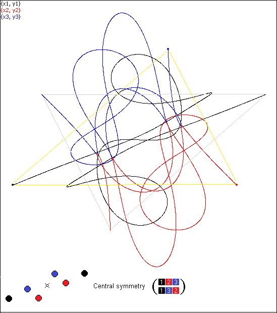
Simulation #14: not only is the second triangle congruent to the first,
but also their respective sides are parallel.
AB = 1,
AC = 0.921456266427119,
BC
= 0.679289996641939
A'C' = 0.999999999906395,
A'B' =
0.921456266288986, B'C' = 0.679289996759996
A'C'/AB =
0.999999999906395, A'B'/AC = 0.999999999850092 , B'C'/BC= 1.00000000017379
Moreover, AB||A'C',
AC||A'B',
BC||B'C'.
The supporting data obtained via the Taylor
Center software
The integration method for the 30 simulations used here was the same modern
Taylor method which was used by the authors in a frame of the so called Clean
Numerical Simulation (CNS) [2] at a super-computer. As the authors wrote in
[2], their implementation of the Taylor method admits arbitrary order and double
precision. They, however, didn't mention what was the order used by them, and
what the double precision means for their super computer.
In this Taylor Center software (also with an arbitrary order) we used the order
30 with maximum precision of float point numbers supported by processors Intel,
which is the 10 byte float type called extended: 63-bit mantissa and
16-bit exponent.
For each of the 30 computed simulations the outputted data is comprised of the
following elements:
- The header containing the sequence # of the simulation, its half-period (taken from [1]), and the number of integration steps;
- The initial lengths of the three edges of the triangle denoted ao1, ao2, ao3 (computed from the coordinates taken from [1]).
- The lengths a1, a2, a3 of the second full stop.
- The "best proportions" between the edge lengths among 3! = 6 possible permutations: "the best" meaning those closest to 1. If neither of the 6 permutation yields the proportions close to three 1s, the message "no congruence" appears.
- The 6 values of components of the velocities in the moment T/2 of the second full stop posted as a proof of reaching this state and the achieved accuracy of the full stop.
If the congruence did take place, the data package contains also:
- The proportions yielding values close to 1, for example
a3/ao1
= 1.00000000202946
a2/ao2 = 0.999999997920113
a1/ao3 = 1.00000000030637
- The 3x3 matrix of angles between the edges ao1, ao2, ao3 and edges a1, a2, a3 in order to see if there are angles close to 0° or 180°, for example
ao1 ao2
ao3
a1 138.847783298464°
179.999999953788° 104.361663992048°
a2 179.999999940341°
138.847783191836° 63.2094472309557°
a3 116.790552658371°
75.6383359097635° 5.33608528907246E-008°
If the angles close to 0° or 180° are detected, the pairs of parallel
edges are displayed.
Here is the actual data obtained with the computer
for the 30 samples.
Notes on accuracy
We see that the proportions expected to be 1, and the velocities expected to be
zero, actually differ from the targeted values. The accuracy of those values
depend on several factors: on the accuracy of the parameters provided by the
author, and on the limits of accuracy in this Taylor integrator.
In the Taylor Center software the accuracy of integration (in ideal cases) may
achieve up to 63 binary digits of the mantissa all being correct at every step,
which corresponds to 18 correct decimal digits. Even with such ultimate 63-bit
accuracy achievable at one step, the global error increases with growing number
of steps (due to the rounding errors, or worse, due to catastrophic subtraction
error in some problems). For example, in a test for simulation #1 integrated
from 0 to its period T and back to 0, the accuracy of the method in
terms of the absolute error was about 10-13 for the positions and 10-12 for the velocities in about 2500 integration steps.
Thinking about the reasons that the actual accuracy of the proportions and
velocities obtained in this numerical experiment is not so good, first
observation is that the values of the initial positions and the periods were
specified by the authors only up to 11 decimal digits (instead of possible 18
in the PCs). Therefore, in order to see whether a more accurate value of the
period T may make the velocities closer to zero at the second rest
position, I resorted to the unique feature of this software – switching
between different independent variables. In so doing, I switched from
integration in independent variable t to integration in the velocity v3 as a new independent variable setting the termination
condition v3 = 0
with the hope that u1, v1, u2, v2, u3, would get
closer to zero. They did not: perhaps it's an insufficient accuracy in the
authors' given initial positions which caused the here observed inaccuracy in
the discussed values.
However, the real breakthrough in the accuracy and search of new cases of the free fall periodic orbits comes with the project [10] performed on a super-computer.
References
1. Xiaoming Li and Shijun Liao, Movies of the Collisionless Periodic
Orbits in the Free-fall Three-body Problem in Real Space or on Shape Sphere http://numericaltank.sjtu.edu.cn/free-fall-3b/free-fall-3b-movies.htm
2. Xiaoming Li and Shijun Liao, Collisionless
periodic orbits in the free-fall three-body problem. https://arxiv.org/pdf/1805.07980.pdf
3. Xiaoming Li, Shijun Liao, Collisionless periodic
orbits in the free-fall three-body problem, https://doi.org/10.1016/j.newast.2019.01.003
4. The Taylor Center software, http://taylorcenter.org/Gofen/TaylorMethod.htm
5. The supporting data http://taylorcenter.org/Workshops/3BodyFreeFall/All30New.htm
6. Resources for the concept and discovery of Choreographies. http://taylorcenter.org/Simo/
7. Resources for the periodic solutions of a plane 3 body problem. http://taylorcenter.org/Hudomal/
8. Resources for the free fall periodic solutions of plane 3 body problem. http://taylorcenter.org/XiaomingLI-ShijunLIAO/
9 .The gallery of 12 high resolution orbits with special properties: http://taylorcenter.org/Workshops/3BodyFreeFall/Congruence/
10. Numerical search for three-body periodic free-fall orbits with central symmetry, by I. Hristov1, R. Hristova1, T. Puzynina2, Z. Sharipov2, Z. Tukhliev (2025)