Unsolved Problems
1) The Conjecture as a gap in the Unifying View and the foundation of Automatic Differentiation
2)
How to establish that (scalar) elementariness of a function is
violated at a certain point
3) A question about the functions having no points of violation of
scalar elementariness
4) Regularization of a polynomial ODE and the Conjecture
5) More suspects for points of violation of elementariness
6) "AD" for singularities: Scenarios of evaluation
of formal derivatives at a singular point of a polynomial m-order ODE
Here and further on we deal with holomorphic functions and their derivatives in
the complex plane.
The Conjecture (a brief presentation here (slides 6-8), in details here) is not the only unsolved problem emerging in the frame of the Unifying View, but it is the central open issue affecting the shape of the Unifying View theory. Below are a few problems topped by the Conjecture proper and including other unsolved problems associated with the Conjecture, all awaiting attention of the mathematical community.
1) The Conjecture as a gap in the Unifying View and the foundation of Automatic Differentiation
In either of the two equivalent forms below, the Conjecture claims that ...
|
For any component, say x(t), of an explicit system in x(t), y(t), z(t), ... of m 1st order rational ODEs
|
For any component, say x(t), of an explicit system in x(t), y(t), z(t), ... of m 1st order polynomial ODEs(1)
regular at all points of its phase space, for any initial point t=a, in particular, having a holomorphic solution x(t) with all its derivatives x(k)(t) |
|
there exists an explicit n-order rational ODE satisfied by x(t)
x(n) = R(t, x, x', x", ..., x(n-1)) (3)
|
|
So far neither the proof nor counterexample for this Conjecture is available. However if the Conjecture is weakened by dropping the requirement of regularity in the target ODE (3), there is a proof based on combinatorial considerations (though impractical for obtaining the target ODE) – see the slide 13 or Appendix 1 here) .
Latest development (2025). In the end of 2022, I drafted a paper believing that I has solved the Conjecture. Soon, however, (prompted by Christer Kiselman), I discovered a mistake in the crucial Lemma. This unpublished manuscript however became available as a preliminary print.
In April 2023, I posted the report on the stumbling block standing on the way of solution of the Conjecture – the exceptional situation at which the earlier attempted proof fails.
In February
2025, I posted the report containing a
limited proof of the Conjecture where that exceptional case remains open. There
is also an extensive discussion outlining the situation when the gap is finally
closed and the Unifying theory completed.
___________________
(1) 1st order rational ODEs
regular at a given point are transformable into a wider polynomial
system of ODEs.
Evolution of the concept of elementary functions
First elementary functions were defined by Liouville in the 19th century as a matter of convention: a few well studied vastly used functions and their finite compositions.
In the 1960s Ramon Moore suggested a different approach, replacing the convention about the elementary functions with a definition based on their fundamental property.
Moore defined (vector-) elementariness based on a property of an elementary vector-function to satisfy a system of explicit rational 1st order ODEs.
A competing definition of stand-alone or scalar elementariness would be based on a property of an elementary function to satisfy one explicit rational ODE of order n, or one implicit polynomial ODE of order n.
The vector elementariness
by Moore easily follows from the scalar elementariness (because conversion of
an n-order ODE into a system of 1st order ODEs is trivial). As to the
vice versa statement, the scalar elementariness by Moore follows from vector
elementariness due to the Theorem proved by me in Appendix 1 here. Therefore the scalar and vector
elementariness by Moore are equivalent.
The Liouville-elementary functions are also Moore-elementary. Say cos t
is vector-elementary together with sin t because they satisfy the system
x' = -y
y' = x .
However, each of them is also scalar-elementary satisfying the ODE x"
= x (or satisfying an implicit
first order non-linear ODE (x')2 + x2
= 1). In general case however it may be a challenge to obtain an n-order
ODE verifying the scalar elementariness from the system of ODEs verifying the
vector-elementariness.
It was understood indeed that there exist infinitely many ODEs for verifying elementariness of a particular (vector-) function: some ODEs possibly singular at certain points of their phase space.
It's worth noting that...
The Moore definition applies to the functions...
· In their entire domain of existence, and ...
· With understanding that the rational ODEs may have points of singularity in their phase space unusable as initial points, though sometimes it's possible to replace singular ODEs with the regular ones at the point of interest.
Then in 2008 it was discovered that there exist isolated points in some holomorphic scalar-elementary functions whose Moore-elementariness at such points may be demonstrated only with singular ODEs. For example, such is the function
|
x(t) = |
et – 1 |
|
t |
x(0) = 1
considered in details below. Such kind of special points were earlier known as "regular singularities" or "removable singularities". As it was shown, though the singularity in functions at such point is removable and the functions are holomorphic (with the proper defined value at such point), it's impossible to rid of singularity in the ODEs demonstrating their Moore-like scalar-elementariness at such points. This new type of specialty happens to be unremovable (discussed in item 2).
It was namely the discovery of these special points which gave the reason to
refine the Moore definition of elementariness as a property of a function at a neighborhood
of a point (rather than a property in the entire domain of existence).
The refined definitions of elementariness
Definition 1: a vector-function (x, y, z, ...) is
called vector-elementary at and near a point t=a if
it satisfies a system of rational ODEs (1) regular at the point t=a, or
a polynomial system (2).
Definition 2: a function x(t) is
called scalar-elementary at and near a point t=a if
it satisfies a rational ODE (3) regular at the point t=a, or if it satisfies an implicit polynomial ODE (4) regular at a
meaning ∂P/∂Xm|t=a ≠ 0 (where Xm denotes
x(m)).
The vector elementariness easily
follows from the scalar elementariness (because conversion of an n-order
ODE into a system of 1st order ODEs is trivial). As to the vice versa
statement, the scalar elementariness would follow from the vector
elementariness if the Conjecture is true. Therefore equivalence between these
two definitions depends on the Conjecture.
Most properties and results in the "Unifying View" are proved
only for vector-elementariness, and it is not known whether they are
true for scalar elementariness. In particular, the fundamental property
of closeness of the class of vector-elementary functions states that a
composition of such vector-functions, or the inverse vector-function preserves
vector-elementariness. (For the scalar elementariness this is not known).
2) How to establish that (scalar) elementariness of a function is violated at a certain point?
Until recently the only function proved to be non-elementary (at all points of its domain!) was the Euler's Gamma function – thanks to the Holder theorem utilizing the special property of the Gamma function to satisfy the finite difference equation Γ(x+1) = xΓ(x).
Our method of proof that scalar elementariness of a function is violated at a
certain point utilizes the specific of the sequence of derivatives at this
point, for example the specific of x(n)|t=0
= 1/(n+1) (see the article
).
Any holomorphic function x(t) is defined entirely by its analytic element, i.e. by the sequence of derivatives x(n)|t=a at a point. It appears that the scalar elementariness at a point a also depends on the property of the sequence of its derivatives x(n)|t=a . For the type of functions and examples considered in the article, the sequences of derivatives are rational numbers x(n)|t=a =rn .
The method of proof is based on considering polynomial ODEs P(t, X, X1,…, Xm)=0 over integer coefficients at a regular point where ∂P/∂Xm =c ≠ 0. By applying differentiation, we may obtain an infinite sequence of polynomial ODEs Pk(t, X, X1,…, Xm,…, Xm+k)=0 and then to establish that for all leading derivatives ∂P/∂Xm+k =c ≠ 0.
As a first step, the study was made for a particular function
|
x(t) = |
et – 1 |
|
t |
where all derivatives exist and x(n)|t=0= 1/(n+1). The idea of the proof was in that while k grows to infinity, the denominator 1/(n+k) passes through all prime numbers. Therefore, for a big enough prime n+k, the fraction 1/(n+k) in the equation Pk =0 cannot cancel with other fractions, leading to a contradiction. That way it was proven that x(t) at t=0 can satisfy no regular polynomial ODE, meaning that its scalar elementariness is violated at t=0 – followed merely from the fact that the sequence of derivatives x(n)|t=a are fractions (in lower terms) with growing denominators!
This observation enabled uncovering a wide class of functions whose sequence of derivatives is also represented by fractions with infinitely growing denominator (see Table 1 in the article), and here are examples of the respective functions all having t=0 as a point of violation of scalar elementariness:
|
|
et – 1 |
|
sin t |
|
ln(t + 1) |
|
cos √t |
|
t |
t |
t |
It's notable that (sin t)/t at t=0 represents the "remarkable limit" (studied in the foundation of the calculus). It's new meaning is that it is a point of violation of the scalar elementariness of the respective entire function. The function (ln (1+t))/t is also closely related to the "remarkable limit" (1+t)1/t (see section 4).
And here comes an unsolved part. There are functions – suspects for having
points of violation of elementariness, whose sequence of fractions representing
the derivatives at the point in question does not fall into the above
pattern of fractions with denominator passing throw all prime numbers. For
example, the family of Bessel functions J(t) satisfies the known ODE
t2x" +
tx'+ (t2 – p2)x=0
singular at t=0, and it is not known whether it satisfies a
regular ODE at t=0. For every function of the Bessel family Jp
the expansion at t=0 is known and its general term is
|
Jp(n) = |
(-1)kCkp+2k |
|
2p+2k |
for n=p+2k, k=0, 1, 2,…, and zero otherwise. However it's impossible to draw a controversy from these fractions following the method of proof above (the denominators are not growing primes).
Do the Bessel functions have violation of scalar elementariness at t=0?
What about points of violation of vector elementariness?
Another unsolved part of the problem is whether the examples of functions above having t=0 as a point of violation of their scalar elementariness violate also their vector elementariness at that point (the answer depending on the equivalency of the two definitions, or on the Conjecture).
3) A question about the functions having no
points of violation
of scalar elementariness
At point t=0, all the functions
above can satisfy no regular rational ODE – and consequently no explicit
polynomial ODE; but which kind of ODEs can they satisfy at points other
than t=0?
Indeed, at points other than t=0 they do satisfy rational
ODEs (or implicit polynomial ODEs). As to explicit polynomial
ODEs, here is
Theorem 1. If a function x(t) has a point of violation of its scalar elementariness, it can satisfy no explicit polynomial ODE
x(n) = P(t, x, x', x", ..., x(n-1)). (5)
The equivalent form of this Theorem is...
Theorem 2. If a function x(t) satisfies an explicit polynomial ODE (5), x(t) is scalar elementary in its entire domain of existence (i.e. it has no points of violation of its scalar elementariness).
However, the vice versa statement is an open Proposition.
Proposition. If a function x(t) is scalar elementary in its entire domain, it must satisfy some explicit polynomial ODE (5) rather than a rational ODE (3).
If a functions x(t) is scalar elementary in the entire domain of its
existence, it means that the denominator g(t, x, x', x",...) in R=f/g
of the rational ODE (3) must never disappear on x(t) in its entire
domain. This seemingly suggests that there must be no denominator at all – as
the image of complex functions usually is the entire complex space including 0
(unless the function is a constant), so that the Proposition seems true. In
reality however...
- Either there is no denominator at all because the rational ODE (3) actually happened to be polynomial – as the Proposition claims;
- Or g(t, x, x', x",...) never reaches zero on x(t) because zero may happen to be the excluded (lacunary) value of g (in accordance with the Picard theorem) – see the Example below. It's because of exactly this possibility the Proposition remains an open statement.
Example. Observing that for the function x(t) = et the lacunar value is zero and x = x' = x", the following ODE takes place
x" = (x')2/x, x(0)=x′(0)=1
and its denominator never disappears on x(t). Though in this trivial
example we do know an alternative simple linear ODE satisfied by x(t)
(in accordance with what the Proposition states), for an arbitrary x(t)
we do not know whether the Proposition is true.
4) Regularization of a polynomial ODE and the Conjecture
First consider these examples.
Example 1. The (entire) function x(t) = tet
satisfies the ODE
tx' – tx – x = 0
(6)
singular at t=0. However, x(t) satisfies
also the ODE
x" – 2x' + x = 0
regular at t=0.
Example 2. The (entire) function x(t) = (et – 1)/t satisfies the ODE
tx'
– tx + x – 1 = 0
(7)
singular at t=0. However, it's proven
that there can not exist a polynomial ODE regular at t=0 satisfied by
this function. Nor can it satisfy a polynomial ODE with a constant
nonzero factor at the leading derivative – because unlike in the Example 1,
here function x(t) does have a point of violation of its scalar
elementariness.
Example 3. Besides the ODE (7), the function x(t) = (et – 1)/t also satisfies the ODE
x"(x – 1)(t – 1) – (tx' – 2x' +
x)(x' – 1)= 0
singular at t=1 (with any initial
value for x, in particular with x(1) = e – 1
corresponding to x(t) in Example 2). At that, this x(t) satisfies
also the ODE (7) regular at t=1 (though singular at t=0).
If we set a goal to rid of singularity at t=1 in the Example 3, ODE
(7) is the answer. (The ODE in Example 3 was obtained in a process of an
intentional "planting" of a singularity into the ODE (7) at t=1
described here).
Now comes a question.
Let a holomorphic function x(t)
satisfy a polynomial ODE over complex coefficients
P(t, x, x', ..., x(m)) = 0
(8)
and P=0 happened to be singular at t=0.
Does a method exist which either offers another poly ODE
Q(t, x, x', ..., x(n)) = 0
satisfied by x(t) but regular at t=0,
or it says that x(t) cannot satisfy any poly ODE (8) regular at t=0.
Here is how this question relates to the Conjecture.
If the Conjecture is true and proved, then the answer to the question is this:
If a function x(t) at t=0 satisfies some polynomial system (2), then a regular replacement Q exists. And if function x(t) at t=0 cannot satisfy the polynomial system (2), then a regular replacement Q does not exist.
5) More suspects for points of violation of elementariness
More suspects for points of violation of
elementariness appear in quite unexpected situations. For example, a
transcendental function y(x) which is a non-trivial solution of the
equation of commuting powers xy=yx also satisfies an ODE which is singular at the
point x=y=e:
y"x2y2(y – x) – (y')3x4 + (y')2x2y(3x – 2y) + y'xy2(3y – 2x) – y4 = 0
and it is not known whether y(x) satisfies a regular ODE at the point x=y=e.
It is proven that y(x) is holomorphic at x=y=e, however no
general term in closed form is known for its expansion (its derivatives at this
point are obtainable only via a complicated recurrent equations) – see the
article.
Does the y(x) have violation of scalar elementariness at x=y=e?
Being singular, at this point this ODE has more
than one solution, being satisfied also by the trivial solution – the identity
function y=x . If it were proven that any ODE satisfied by the
nontrivial solution y(x) is satisfied also by the trivial one (thus
having more than one solution), that would prove that x=y=e is really the
point of singularity of the ODE, thus the point of violation of the scalar
elementariness of the nontrivial y(x). However, this is not proved.
Note, that the ODE y'=1 satisfied by the trivial solution is not
satisfied by the nontrivial one.
Amazingly, a similar open question exists concerning the equation of the associating powers x^(y^z) = (x^y)^z. It's solution y = z1/(z – 1), y(1) = e is proved to be holomorphic at the point z = 1. However, it's not known if this is a point of violation of scalar elementariness.
There is another unsolved problem associated with the commuting powers: the function y(x) happens to be closely approximated by a hyperbola (in red)
|
h(x) = 1 + |
(e – 1)2 |
|
x – 1 |
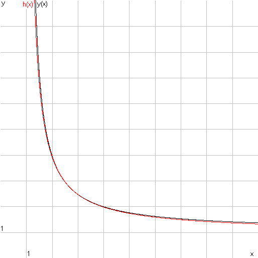
and it was proved that h(x) ≤ y(x) in a small neighborhood of the point x=e. (The proof for all x>1 was recently obtained by Lajos L?czi – August 2020).
6) "Automatic Differentiation" for singular expressions
or
scenarios of evaluation of formal derivatives at a singular point of a
polynomial m-order ODE.
As we saw above, a function f(t) holomorphic at some point t=t0 however may be given with an expression having a removable singularity at this point so that f(t0) must be specially defined as the lim f(t) when t→t0 . Moreover, at certain points (where elementariness is lost) such functions can be defined only via singular rational expressions or ODEs.
Thus, we have holomorphic functions at a point, having all their derivatives,
but the conventional AD is inapplicable for computing those derivatives.
Therefore, we developed a process (as a generalization of AD) capable to
compute n-order derivatives of singular expressions or singular ODEs.
Understandably, the AD generalized for singularities, is more complicate and
less suitable for automatization. That is why the expression "Automatic
Differentiation" is taken in quotes in the title. Unlike at a regular
point, evaluation of ODEs at the singular points admits a variety of scenarios,
which I first outlined in 2009, here in section
8.2.
All cases when an elementary function in question x(t) is defined via
elementary systems of ODEs or expressions containing singularities may be
reduced to one implicit irreducible polynomial ODE
P(x(m) …, x', x, t) = 0
singular at some point t = a, (i.e. ∂P/∂Xm = 0 at t = a). The solution x(t) may or may not exist at this point, or may be not unique.
At a singular point we speak about a process of formal evaluation of the derivatives, and this process may have different outcomes outlined below.
The formal evaluation means applying the rules of differentiation to the
source ODE
.png)
step by step not even expecting that the solution exists and has (complex) derivatives.
After every next n-differentiation, we obtain a more and more cumbersome polynomials Pn (x(m+n), x(m+n - 1), …, x, t). At that, we must check if Pn did not become reducible, and reduce it, if it was the case. For example, if the source ODE is P = (x')2 + x2 – 1 = 0, singular at the point where x' = 0, then after first differentiation, in this case it happens that we obtain a reducible ODE
P1 = 2x'x" + 2x'x = 2x'(x" + x).
Eliminating the factor 2x', we make it a regular ODE x" + x = 0 so that since this moment, the further differentiation behaves like that for a regular ODE.
This process creates an infinite generating system for obtaining a vector of
the formal derivatives x(m+1), x(m+2),….
Both in regular and singular cases the generating system is a triangular
system.
In the regular case the generating system is linear, delivering a unique
solution-vector of "true" derivatives (x, x', x",…, x(m),
x(m+1),…) for the unique holomorphic
solution x(t).
In the singular case the scenario becomes much more complicated as it is
displayed in the table below. If the process for evaluation of formal
derivatives does not stop, the result of the generation is a finite or infinite
set of solution vectors S ={(x, x', x",…, x(m), x(m+1)
,…)} comprised of formal derivatives allowing to write down the
respective formal Taylor expansions (having zero or non-zero convergence
radius). This set S has a sophisticated tree-like structure showed in
the following Table 2.
|
At a regular point... |
At a singular point... |
|
The unique holomorphic solution x(t) exists, its Taylor expansion converges, and its Taylor coefficients comprise the unique solution-vector of the generating system. |
A holomorphic solution of the ODE does not necessarily exist. |
|
The generating system has a unique solution-vector representing the derivatives x(n) of the solution x(t). |
The generating system may have no solution-vectors, or have more than one, or infinitely many of them. |
|
The generating system is triangular, whose each equation is linear in one unknown with the same nonzero coefficient at every unknown. |
The generating system is triangular but not necessarily linear as each of its equations in one unknown is polynomial with numeric or parametric coefficients. |
|
|
Some of the equations may degenerate into a numeric relation true or false. If n-th numeric relation is false, the respective branch of the tree ends (marked by stop). If n-th numeric relation is true (i.e. a zero identity), the respective unknown is a free parameter (like c(m+2)). |
|
If one or several unknowns in the previous equations are free parameters, the subsequent equations become nonlinear polynomial equations with parametric (rather than numeric) coefficients, so that generally it gets impossible to numerically explore and evaluate them. |
|
|
If the set of the solution-vectors of the generating system is non-empty, some or all of the vectors still may comprise a divergent Taylor series (with zero radius) representing no solution. |
Table 1
This table below illustrates an example of evaluation of a polynomial ODE at a
singular point when all polynomials Pn happen to be
irreducible. (If any of polynomials Pn happen to be reducible,
each of its factors must be viewed as a new ODE making a new branch of this
tree).
|
|
The values of the formal derivatives obtainable from the equations of the generating system |
||||||||||||||
|
x |
x, x', x",
.... , x(m) are given. |
||||||||||||||
|
x' |
|||||||||||||||
|
x" |
|||||||||||||||
|
… |
|||||||||||||||
|
x(m) |
|||||||||||||||
|
x(m+1) |
a1(m+1)
The equation in one unknown x(m+2) happened to be of degree 2 having 2 roots a1(m+2), a2(m+2) |
a2(m+1)
The equation in one unknown x(m+2) degenerated into an identity so that x(m+2) may be an arbitrary complex number c(m+2) |
a3(m+1) |
||||||||||||
|
x(m+2) |
a1(m+2) |
a2(m+2) The equation in one unknown x(m+3) happened to be of degree 3
|
c(m+2) The equation in one
unknown x(m+3) |
a3(m+2) |
a4(m+2) |
||||||||||
|
x(m+3) |
stop
|
a1(m+3) |
a2(m+3) |
a3(m+3) |
|
a4(m+3)(c(m+2)) |
a5(m+3)(c(m+2)) |
a6(m+3)(c(m+2)) |
|
|
a7(m+3) |
a8(m+3) |
a9(m+3) |
a10(m+3) |
|
|
... |
… |
… |
… |
… |
… |
… |
… |
… |
… |
… |
… |
… |
… |
||
Table 2
Here x, x', … , x(m) are given as the initial values, while x(m+1), x(m+2),… are to be obtained in the process of solution of algebraic equations in one unknown of some degree k ≥ 0. If k=0 the respective equation degenerated into a numeric relation true or false. If false, this branch ended with a controversy. If true, this equation does not yield a specific solution value allowing the respective x(n) be an arbitrary constant (like c(m+2)). Therefore, the set of branches growing from every node of the tree is either…
- empty (end of the branch), or…
- an infinite uncountable set of the power continuum, or…
- a finite set with the number of branches k representing k different roots of the respective algebraic equation.
I have illustrative examples for many (though not all) cases of this evaluation scenario.
Where (in which textbook or monograph) is this setting and scenario considered?
The answer was delivered by Copilot in 2026.
1. It was considered by Ritt–Kolchin differential algebra (1930s–1970s).
At a point where ∂P/∂x(n) = 0, the prolongation may:
· produce new constraints of lower order,
· produce new constraints of higher order,
· branch into multiple possible formal expansions,
· or become inconsistent.
Who explicitly analyzed this branching?
Joseph Fels Ritt
Differential Algebra (1932), Integration in Finite Terms (1948). He introduced the idea of singular differential polynomials and the behavior of their prolongations.
Ellis Kolchin
Developed the full structure theory of differential ideals, including:
· singularities of differential polynomials,
· differential dimension,
· characteristic sets,
· and the behavior of prolongations when leaders vanish.
2. The analytic tradition: Painleve, Gambier, Chazy (1890–1910)
These authors studied movable singularities of nonlinear ODEs by expanding solutions in Laurent or Puiseux series.
Why they are relevant
When the leading coefficient vanishes, the recursion for coefficients in a formal series becomes:
· underdetermined,
· overdetermined,
· or branching.
This is the same phenomenon you're describing, but approached analytically rather than algebraically.
Key idea
The Painleve test is exactly a branching formal evaluation of derivatives when the ODE becomes singular.
Summarily:
Algebraic viewpoint (closest to your formulation):
· Joseph Fels Ritt
· Ellis Kolchin
Analytic viewpoint (series expansions at singular points):
· Painleve
· Gambier
· Chazy
Geometric viewpoint (implicit ODE singularities):
· Harley Flanders
· Arnold, Davydov, Remizov
DAE viewpoint (hidden constraints via differentiation):
· Kunkel & Mehrmann
· Gear & Petzold
All of them, in different languages, studied the same phenomenon:
When the leading derivative coefficient vanishes, the prolongation tree becomes non-unique, and the structure of possible jets becomes a branching algebraic variety.